5. The Astronomical Pacemaker
We have now arrived at a point where the logical next
question is: Were the monsoonal maximum and the associated eastern Mediterranean
anoxic event of 9,500 to 6,000 years BP unique events in earths history?
As the reader will have deduced from my various references to such events
in the more distant past, the answer to this question is NO. In fact, sapropel
formation has been occurring on a regular basis since about 3 million years
ago, and intermittently even since 9 million years BP. I have also mentioned
before that the pacemaker governing the regular recurrence of monsoonal
maxima is rooted in astronomical cycles. To understand how this works,
we need to explore in what manner astronomical cycles may regulate large-scale
climate variations on earth.
Climate is sensitive to both the total amount, and the
latitudinal and seasonal distribution, of solar radiation onto the earths
surface. Three astronomical cycles are of relevance to these aspects: the
eccentricity cycle, the obliquity cycle, and the precession cycle (note
8). The Serbian engineer Milutin Milankovitch was the first to calculate
in detail the temporal fluctuations in the intensity and distribution of
solar radiation onto the earths surface. His results were presented in
several major publications between 1912 and 1941. One of Milankovitchs
special contributions comprised the determination of past insolation variations
for various discrete latitude bands. In the scientific community concerned
with climates of the past, the three main astronomical cycles are often
referred to as the Milankovitch cycles. From especially the 1970s onwards,
the astronomical calculations have been continuously improved and
updated.
5.1. Eccentricity and Precession
Before these cycles can be discussed, we should refresh our
concepts of what exactly determines the seasonal cycle. The period of one
year marks the time needed for the earth to complete one rotation around
the sun. On such time-scales, the position of the earths rotational axis
relative to the plane of the earths orbit around the sun is fixed in space,
with the North Pole today pointing towards the star Polaris. Consequently,
there is a season in which one of the Poles is tipped away from the sun
(winter hemisphere), while the other Pole is in a direction facing the
sun (summer hemisphere). Six months later, this situation is exactly reversed.
Lets follow one rotation, within a northern hemispheric
(boreal) context (note
9). We start at the boreal winter solstice, the shortest day on the
northern hemisphere when the North Pole is turned directly away from the
sun. The boreal winter solstice marks the start of winter on the northern
hemisphere. The next notable point along the earths orbit is the boreal
spring (vernal) equinox, the start of boreal spring. During an equinox,
day and night at all points of the world have identical durations because
the two Poles are on identical distances from the sun. In other words,
the boundary between the illuminated and dark half-globes passes through
both Poles. Half a year after the winter solstice, the earth reaches the
boreal summer solstice, the longest day on the northern hemisphere, when
the North Pole lists directly towards the sun this marks the start of
boreal
summer. Next, the boreal autumnal equinox is reached, marking the start
of boreal autumn.
 Figure 5. Schematic presentation of a seasonal cycle. Note the importance
of the fixed direction in space of the rotation axis on these short time
scales (today towards Polaris): if the axis were not tilted relative to
the plane of orbit, then there would be no seasons. Click on thumbnail
for full-sized jpeg image (or here
for a pdf).
Figure 5. Schematic presentation of a seasonal cycle. Note the importance
of the fixed direction in space of the rotation axis on these short time
scales (today towards Polaris): if the axis were not tilted relative to
the plane of orbit, then there would be no seasons. Click on thumbnail
for full-sized jpeg image (or here
for a pdf).
The eccentricity cycle concerns variations in the shape
of the earths orbit around the sun. This shape varies from near circular
to distinctly elliptical (oval shaped). An ellipse has two focal points,
and as the ellipse transforms to a circle, the two focal points approach
one another. When a perfect circle is formed, the two focal points overlap
and define the centre-point of the circle. The sun occupies one of the
focal points of the earths orbit. Therefore, in an eccentricity maximum
(strong ellipse), the earth in one of its yearly revolutions around the
sun passes a point where it stands nearest the sun (at perihelion) and
a point where it stands furthest away from the sun (at aphelion). When
the orbit is near circular an eccentricity minimum the earths distance
to the sun is virtually constant through the year. The eccentricity of
the earths orbit changes in a cyclic fashion, with three main periods:
94,800 years, 123,800 years, and 404,000 years. These are often approximated
in studies of past climates by using apparent periods of 100,000 and 400,000
years.
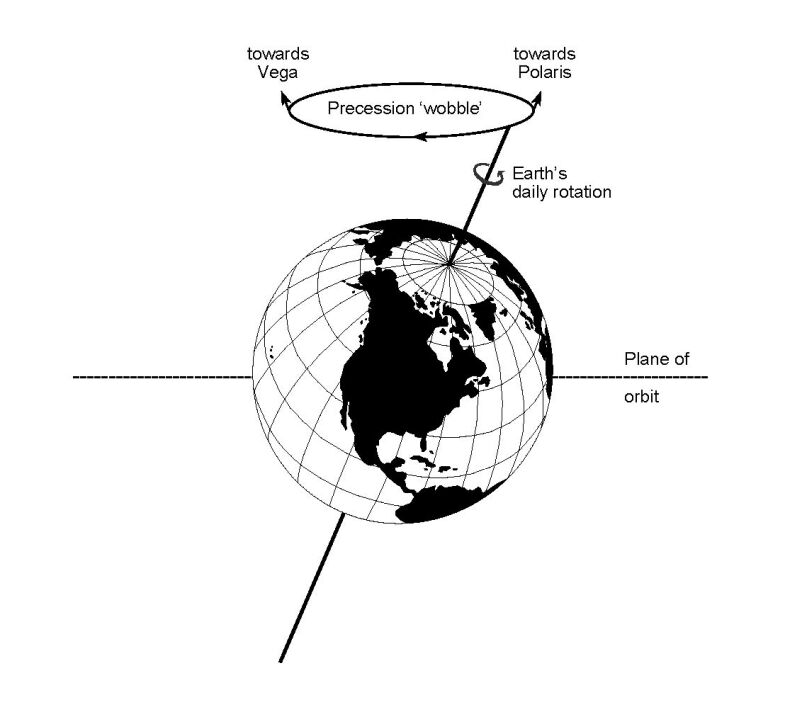
Another very important cycle for climate is that of precession.
The precession cycle is related to the fact that the earths rotational
axis relative to the plane of the earths orbit around the sun on the long
term is not fixed in space, but wobbles like the axis of a spinning top.
Here, we are not talking about changes in the angle of the axis relative
to the plane of orbit (which is discussed below under obliquity or tilt),
but about changes in the direction of the axis in space. Essentially, the
precession cycle causes the North Pole, which today points towards Polaris,
to point towards Vega (which then becomes the North Star) after half a
precession cycle, and back towards Polaris again after a complete precession
cycle. A full cycle of precession takes 26,000 years. However, other complications
in the earth-sun motions come into play the entire earth orbit itself
slowly rotates around the sun, about once for every four precession periods.
As a result, the precession cycle manifests itself in the insolation
onto the earths surface in two dominant periodicities; a major one centered
on 23,000 years (23,700 and 22,400 years to be precise) and a minor one
of 19,000 years. As a first-order approximation, some people like to use
an average periodicity of 22,000 years.
The precession cycle affects climate by causing a very
slow shifting of the dates of the solstices and equinoxes along the orbit.
A quarter of a cycle ago (about 5,500 years BP), therefore, perihelion
occurred near to the boreal autumnal equinox. Half a cycle ago (about 11,000
years BP), perihelion occurred close to the boreal summer solstice. Three
quarters of a cycle ago (about 16,500 years BP), perihelion coincided with
the boreal vernal equinox, and a full cycle ago the situation concerning
precession was similar to the present.
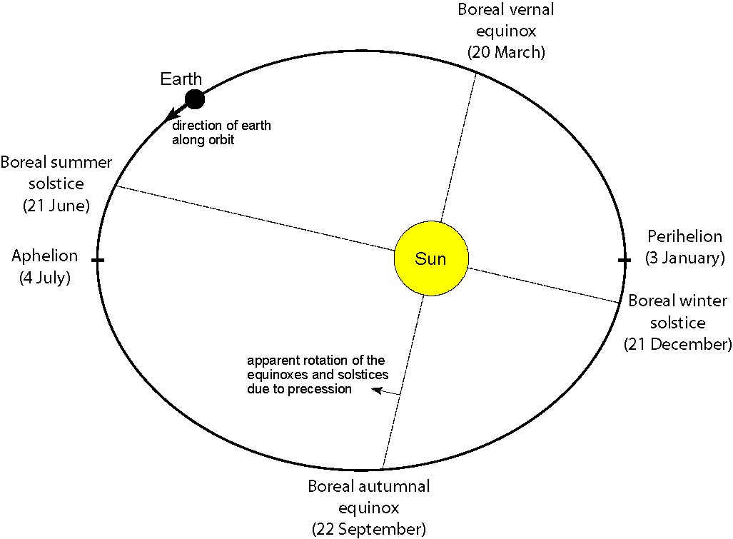
 Figure 6. Schematic presentation of a top view of earths orbit around
the sun (not to scale). Also indicated are the current dates at which the
earth reaches the solstices and equinoxes, and the dates at which it reaches
aphelion and perihelion. The direction is given of the shift along the
orbit of the solstices and equinoxes, caused by precession. Click on thumbnail
for full-sized jpeg image (or here
for a pdf).
Figure 6. Schematic presentation of a top view of earths orbit around
the sun (not to scale). Also indicated are the current dates at which the
earth reaches the solstices and equinoxes, and the dates at which it reaches
aphelion and perihelion. The direction is given of the shift along the
orbit of the solstices and equinoxes, caused by precession. Click on thumbnail
for full-sized jpeg image (or here
for a pdf).
 Figure 7. The earths precession wobble. One revolution takes 26,000
years.Click on thumbnail for full-sized jpeg
image (or here for a pdf).
Figure 7. The earths precession wobble. One revolution takes 26,000
years.Click on thumbnail for full-sized jpeg
image (or here for a pdf).
The climatic impacts of the precession and eccentricity
cycles need to be viewed together. Today, in its slightly elliptical orbit,
the earth is at perihelion around the boreal winter solstice 3 January
and 21 December, respectively. This implies that it is at aphelion around
the boreal summer solstice 4 July and 21 June, respectively. When the
orbit approaches a circle, these distance differences would have negligible
effects. However, since some eccentricity applies, the solar radiation
on illuminated places of the globe will be somewhat more intense in boreal
winter (austral summer) than in boreal summer (austral winter). Effectively,
this weakens the northern hemispheres seasonal contrast, whereas that
on the southern hemisphere is strengthened. The precession cycle, meanwhile,
causes shifts in the distribution of the seasons around the elliptical
orbit. Half a precession cycle ago, therefore, the situation would have
been the reverse of that observed today, with perihelion near the boreal
summer solstice and aphelion around the boreal winter solstice. That configuration
would enhance the seasonal contrast on the northern hemisphere.
Summarising, the precession cycle governs the seasonal
insolation contrast, but its impact depends on the degree of eccentricity
of the orbit. In a circular orbit the precession cycle has no impact, while
in times of maximum eccentricity the precession cycle reaches maximum impact.
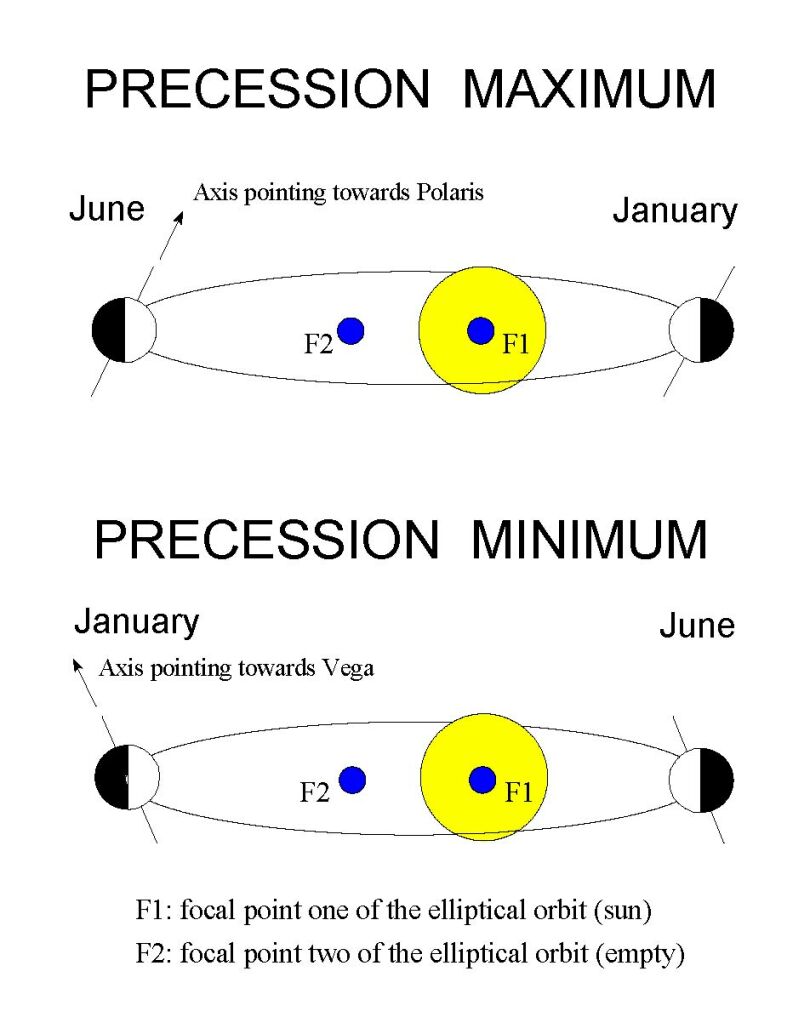
 Figure 8. Summary schematic to demonstrate the differences between
precession maxima (as today) and precession minima. Note the exaggerated
eccentricity of earths orbit with two focal points, of which one occupied
by the sun. The direction in space of the earths axis has changed from
pointing towards Polaris in the precession maximum, to pointing towards
Vega in the precession minimum.Click on thumbnail for full-sized
jpeg image (or here for a pdf).
Figure 8. Summary schematic to demonstrate the differences between
precession maxima (as today) and precession minima. Note the exaggerated
eccentricity of earths orbit with two focal points, of which one occupied
by the sun. The direction in space of the earths axis has changed from
pointing towards Polaris in the precession maximum, to pointing towards
Vega in the precession minimum.Click on thumbnail for full-sized
jpeg image (or here for a pdf).
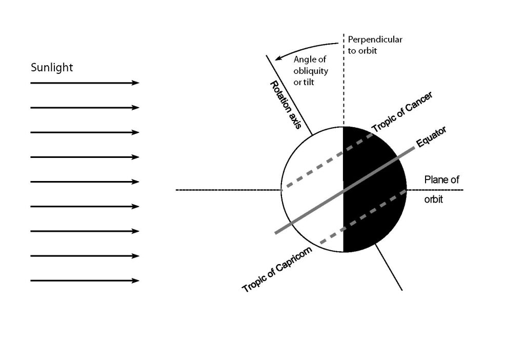
5.2. Obliquity
The cycle of obliquity concerns a gradual change in the angle
of the earths rotation axis relative to the perpendicular of the plane
of the earths orbit. This angle changes from 22.5 to 24.5 degrees and
back again over a period of 41,100 years. Today, the angle is about 23.5
degrees. As a consequence, the sun during the boreal summer solstice stands
directly overhead at about 23.5º North latitude, which represents
the maximum North latitude where the sun at any one time in the year reaches
a directly overhead position. This latitude is called the Tropic of Cancer.
During the boreal winter solstice (austral summer solstice) this condition
is reached at about 23.5º South latitude the Tropic of Capricorn.
On a perfectly spherical earth, the obliquity cycle would therefore shift
the position of the Tropics between 22.5 and 24.5º latitude the
actual values are 22.04 and 24.45º. In addition, the obliquity (or
tilt) of the axis affects the amount of sunlight received at the high
polar latitudes. For strong tilt, the poles receive more sunlight, and
the suns rays also reach the polar surface at a less shallow angle, which
decreases their reflection and so increases the heat absorption.
 Figure 9. The relationship between obliquity, or tilt, and the positions
of the Tropics of Cancer and Capricorn. The tilt of the earths axis relative
to the perpendicular to the orbital plane varies on a 41,100 years cycle
between about 22.5 and 24.5 degrees. Today, the tilt is about 23.5 degrees.
For clarity, the angle is exaggerated in this diagram.Click on thumbnail
for full-sized jpeg image (or here
for a pdf).
Figure 9. The relationship between obliquity, or tilt, and the positions
of the Tropics of Cancer and Capricorn. The tilt of the earths axis relative
to the perpendicular to the orbital plane varies on a 41,100 years cycle
between about 22.5 and 24.5 degrees. Today, the tilt is about 23.5 degrees.
For clarity, the angle is exaggerated in this diagram.Click on thumbnail
for full-sized jpeg image (or here
for a pdf).
5.3. Monsoonal Maxima and Sapropels
The first comprehensive description of the relationship between
monsoonal maxima and associated sapropel formation, and the astronomically
determined insolation cycles was pioneered by the French specialist in
reconstructions of climatic impacts on past vegetation (paleo-botanist)
Martine Rossignol-Strick. She approached the problem by specifying an index
for monsoon intensity (monsoonal index) as a function of two parameters:
one was the insolation at the Tropic of Cancer, and the other was the difference
in insolation at the Tropic of Cancer and at the equator. Note that insolation
is by convention measured at the top of the atmosphere. The astronomical
calculations for insolation at the various latitude bands on earth showed
that insolation variations in the low latitudes are strongly dominated
by the precession cycle. This implies that also the eccentricity cycle
is very important, since the intensity of the precession influence depends
on eccentricity. Obliquity influences were found to be rather weak at low
latitudes, but very important at higher latitudes.
Martine Rossignol-Stricks work, which concentrated on
the last half million years, started an intensive search into the timing
of sapropel formation over their full temporal range. It has since been
confirmed that the sapropels were always associated with times when perihelion
falls in boreal summer (precession minima, relative to maxima that
represent the present configuration with perihelion in boreal winter).
In addition, it was observed that not all precession minima have sapropels,
but that they instead occur in discrete clusters. Each cluster was found
to represent times of maximum orbital eccentricity. This makes sense, since
eccentricity maxima are times when the effects of the precession cycle
on insolation are strongest.
So how does precession influence the monsoon? The key
issue here concerns its impact on seasonal contrasts. Another important
factor to take into account is the strong oceanland alternation on the
northern hemisphere, which contrasts with the much more ocean dominated
southern hemisphere. As this book concerns processes on the northern hemisphere,
the following discussion uses summer for the northern hemisphere (boreal)
summer, and winter for the boreal winter unless indicated otherwise.
During precession minima, perihelion occurs in summer,
causing enhanced summer insolation. Aphelion falls in winter, causing reduced
winter insolation. The seasonal insolation contrast, therefore, is considerably
higher during a precession minimum than today (near a precession maximum).
This affects land and ocean in different ways, since land has negligible
thermal inertia compared with ocean water. In other words, land heats up
and cools down very rapidly: enormous day-night contrasts demonstrate this,
with extremes reaching from +50 to 5ºC in subtropical deserts. This
rapid response is reflected in the longer term, with winter heat loss from
land surfaces completely compensating for all summer heat gain. In contrast,
it takes considerable time for the ocean to warm up and cool down. Day-night
temperature fluctuations in the upper ocean consequently are generally
1ºC or less (down to 0.1ºC), with a large part of this stability
related to continuous mixing processes within the surface mixed layer (note
10).
Atmospheric surface pressure responds to temperature fluctuations,
since air over a hot surface rises, giving low surface pressure, while
it descends over a cool surface, giving high surface pressure. As a result,
land surfaces experience a much stronger annual fluctuation in both temperature
and pressure than ocean surfaces (note
11). During periods with enhanced seasonal insolation contrasts, the
higher summer insolation increases the surface temperatures especially
over land, which in turn amplifies the atmospheric pressure differences
between land and sea. In addition to this direct radiative forcing, the
preceding winter conditions also play a role, due to the thermal inertia
of the ocean. The slow response of oceanic temperatures on seasonal time
scales amplifies the land-sea temperature contrast from direct solar heating,
and thus enhances the land-sea pressure differences.
In summer, the strong land (low) to sea (higher) pressure
difference leads to surface air flow from ocean to land. This air flow
is moisture laden, because of evaporation over the ocean. The air expands
and cools as it rises over the land, a process that is accellerated if
the air masses are forced up by mountain ridges. Cool air can carry less
vapour than warm air, and the cooling causes the air-masses to shed their
vapour as rain. Condensation releases heat, which amplifies the process
by enhancing the ascending motion in the air column. Thus, a zone develops
of high-frequency and high-intensity monsoonal rains.
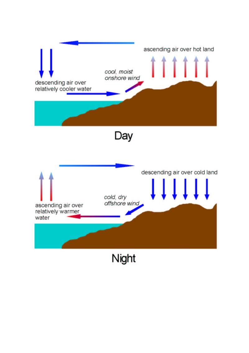
 Figure 10. Schematic presentation of the sea breeze effect (see footnote
11), which is often used as an illustration of a purely thermally forced
monsoon (day then is summer, night serves to illustrate the winter). Although
monsoons in reality are more complicated than this, the thermal monsoon
serves as a useful concept in miniature for the African monsoon. Note that
the overland ascent of moist oceanic air in the day/summer configuration
is likely to fuel convective rainfall (in the sea breeze context, this
leads to the common heavy rains observed in tropic islands just after the
hottest time of day). Click
on thumbnail for full-sized jpeg image (or
here
for a pdf).
Figure 10. Schematic presentation of the sea breeze effect (see footnote
11), which is often used as an illustration of a purely thermally forced
monsoon (day then is summer, night serves to illustrate the winter). Although
monsoons in reality are more complicated than this, the thermal monsoon
serves as a useful concept in miniature for the African monsoon. Note that
the overland ascent of moist oceanic air in the day/summer configuration
is likely to fuel convective rainfall (in the sea breeze context, this
leads to the common heavy rains observed in tropic islands just after the
hottest time of day). Click
on thumbnail for full-sized jpeg image (or
here
for a pdf).
It needs to be noted that the above description of the
summer monsoon, centered on surface thermal forcing, represents a rather
simplified generalisation. In reality, the low pressure cell over land
cannot reach the required intensity, nor the continuity, without strong
assistance by dynamical effects related to the mean high-level wind flow
in the atmosphere (at the 500 millibar level, or approximately at 5.5 km
height). As an extra complication, it is thought that the strength of the
trade winds on the opposite (winter) hemisphere may determine a push
across the equator into the summer monsoonal low.
Despite its schematic nature, the thermal concept offers
a rather nice representation of the general features of the African monsoon (note
12). Over Africa, the axis of low pressure at the surface (the monsoonal
low-pressure trough) follows the seasonal march of the sun at its high
point (zenith), which reaches the Tropic of Cancer at the summer solstice.
This seasonal swing over the band of monsoonally influenced latitudes in
Africa can be so smooth because most of Sahelian and Saharan North Africa
consists of relatively flat lowlands. The influence of push effects
by the southern (winter) hemisphere trade winds on the North African summer
monsoon was included in the monsoonal intensity index by inclusion of an
austral winter insolation gradient. This gradient was used as a first-order
measure of the thermal contrast on the southern winter hemisphere that
affects the trade wind intensity.
The above conceptually relates the intensity of the summer
monsoon to the insolation cycles. So, what about the expansion of
the summer monsoon over a far more extensive area than today, with strong
northward penetration over Africa? Firstly, a dramatic increase in monsoon
intensity by itself would arguably shift its impact on vegetation and other
humidity markers somewhat to the north. Secondly, and more importantly,
the expansion is also affected by the insolation variations, but then in
particular by changes in the structure of the latitudinal insolation gradients.
Comparison of records of insolation variations for several latitude bands
with present-day insolation values at the same latitudes shows that the
maximum increase in insolation, relative to the present, has shifted north
and south over the tropical latitudes. Maximum monsoon expansions occurred
when this maximum increase was located at higher tropical latitudes. An
important control on the latitude of maximum insolation change relative
to the present is determined by the obliquity cycle. As the tilt of the
earths axis relative to the orbit increases, both Tropics shift to higher
latitudes, while a decrease of tilt causes both Tropics to shift to lower
latitudes.
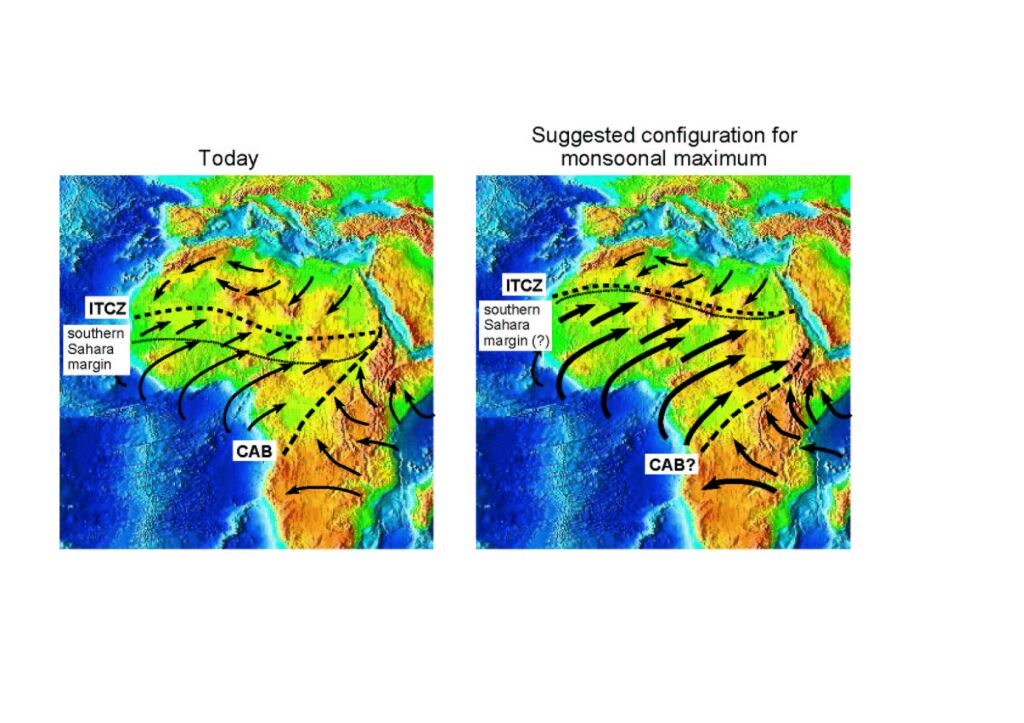
 Figure 11. Rough locations of the Intertropical Convergence Zone
(ITCZ), the Congo Air Boundary (CAB), and the southen margin of the Sahara
Desert for the present-day, and in an artists interpretation for the
monsoonal maximum. The ITCZ is the area of maximum ascent in the air column
(hence air is being drawn into this zone from both the south and the north).
This zone follows the thermal equator over N Africa. Therefore, the representation
above is for the time around the boreal summer solstice, when the sun reaches
is northernmost position. The CAB represents the boundary between airmasses
originating from the Atlantic and Indian Oceans.Click on thumbnail for
full-sized
jpeg image (or here for a pdf).
Figure 11. Rough locations of the Intertropical Convergence Zone
(ITCZ), the Congo Air Boundary (CAB), and the southen margin of the Sahara
Desert for the present-day, and in an artists interpretation for the
monsoonal maximum. The ITCZ is the area of maximum ascent in the air column
(hence air is being drawn into this zone from both the south and the north).
This zone follows the thermal equator over N Africa. Therefore, the representation
above is for the time around the boreal summer solstice, when the sun reaches
is northernmost position. The CAB represents the boundary between airmasses
originating from the Atlantic and Indian Oceans.Click on thumbnail for
full-sized
jpeg image (or here for a pdf).
(Background
topographic map developed by Marine Geology and Geophysics Division
of the National Geophysical Data Center, Copyright
© 1989 by Jef Poskanzer).
To Chapter 6
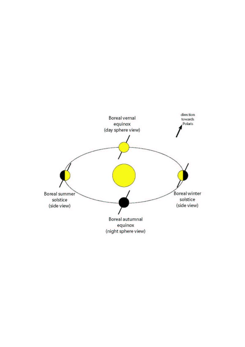 Figure 5. Schematic presentation of a seasonal cycle. Note the importance
of the fixed direction in space of the rotation axis on these short time
scales (today towards Polaris): if the axis were not tilted relative to
the plane of orbit, then there would be no seasons. Click on thumbnail
for full-sized jpeg image (or here
for a pdf).
Figure 5. Schematic presentation of a seasonal cycle. Note the importance
of the fixed direction in space of the rotation axis on these short time
scales (today towards Polaris): if the axis were not tilted relative to
the plane of orbit, then there would be no seasons. Click on thumbnail
for full-sized jpeg image (or here
for a pdf).